Decoding The Skew-T Log-P Diagram: A Complete Information

Decoding the Skew-T Log-P Diagram: A Complete Information

Associated Articles: Decoding the Skew-T Log-P Diagram: A Complete Information

Introduction

On this auspicious event, we’re delighted to delve into the intriguing matter associated to Decoding the Skew-T Log-P Diagram: A Complete Information. Let’s weave attention-grabbing data and provide contemporary views to the readers.

Decoding the Skew-T Log-P Diagram: A Complete Information

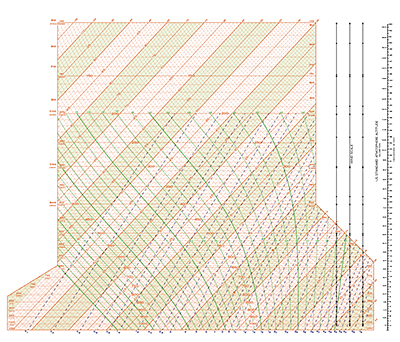
The Skew-T Log-P diagram, a staple in meteorology, is a thermodynamic diagram used to symbolize the vertical profile of atmospheric temperature, humidity, and stability. Its seemingly complicated look belies a strong device for understanding atmospheric processes, essential for climate forecasting and evaluation. This complete information will unravel the intricacies of the Skew-T Log-P diagram, offering a step-by-step strategy to studying and deciphering its data.

Understanding the Axes and Coordinates:

The Skew-T Log-P diagram’s energy lies in its cleverly designed axes. As an alternative of utilizing linear scales for strain and temperature, it makes use of a logarithmic scale for strain and a skewed scale for temperature.

• Strain (P): The vertical axis represents strain, usually starting from 1000 hPa (millibars) on the backside to 100 hPa on the prime. This logarithmic scale compresses the upper altitudes, permitting for a greater illustration of the troposphere and decrease stratosphere on a manageable chart. Every line represents a selected strain stage, essential for figuring out atmospheric layers.

• Temperature (T): The horizontal axis, nevertheless, shouldn’t be a easy linear temperature scale. It is skewed, which means the isotherms (traces of fixed temperature) are slanted. This skewing is designed to enhance the readability of sure thermodynamic processes, significantly these associated to adiabatic processes (processes occurring with out warmth trade with the environment). Isotherms are normally introduced in Celsius or Fahrenheit.

• Skew Angle: The angle of the skew is often round 45 levels. This angle is chosen to optimize the illustration of adiabatic lapse charges (the speed at which a parcel of air cools because it rises). Dry adiabatic lapse charges seem as straight traces on the skew-T, simplifying their identification.

Key Strains and Curves on the Skew-T:

Past the strain and temperature axes, a number of key traces and curves improve the diagram’s utility:

• Isotherms (Strains of Fixed Temperature): As talked about, these are slanted traces representing fixed temperatures. They’re essential for figuring out temperature gradients and figuring out temperature inversions (layers the place temperature will increase with top).

• Isopleths (Strains of Fixed Mixing Ratio): These curves symbolize fixed values of blending ratio (the mass of water vapor per unit mass of dry air). They’re essential for understanding humidity profiles. Increased values point out extra moisture within the air.

• Dry Adiabats (Strains of Fixed Dry Adiabatic Lapse Fee): These are straight traces representing the speed at which a parcel of dry air cools because it rises adiabatically (with out warmth trade). This lapse fee is roughly 9.8 °C per kilometer.

• Moist Adiabats (Strains of Fixed Moist Adiabatic Lapse Fee): These curves symbolize the speed at which a saturated parcel of air cools because it rises adiabatically. The moist adiabatic lapse fee is lower than the dry adiabatic lapse fee as a result of latent warmth is launched throughout condensation. These curves are essential for understanding cloud formation and precipitation.

• Saturation Mixing Ratio (Saturation Curve): This curve represents the utmost quantity of water vapor that the air can maintain at a given temperature and strain. Air above this curve is saturated, whereas air under is unsaturated.

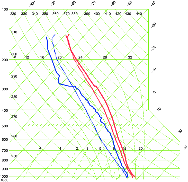
Decoding Soundings:

A sounding is a vertical profile of atmospheric situations obtained from climate balloons carrying radiosondes. This information is then plotted on the Skew-T Log-P diagram. Decoding a sounding includes understanding a number of key elements:

1. Temperature Profile: Plot the temperature information factors onto the diagram. Join these factors to create the temperature profile. Observe the temperature gradient – is it secure (temperature reducing with top), conditionally unstable (temperature reducing at a fee between dry and moist adiabatic lapse charges), or unstable (temperature reducing at a fee quicker than the dry adiabatic lapse fee)?

2. Dew Level Profile: Plot the dew level information factors. The dew level is the temperature at which the air turns into saturated. The distinction between the temperature and dew level is the dew level melancholy. A small dew level melancholy signifies excessive humidity.

3. Figuring out Lifting Condensation Degree (LCL): The LCL is the altitude at which a parcel of air, lifted adiabatically, turns into saturated. It is discovered by drawing a dry adiabat from the floor temperature and dew level intersection till it intersects the saturation mixing ratio curve.

4. Figuring out Degree of Free Convection (LFC): The LFC is the altitude at which a lifted parcel turns into hotter than its environment, initiating free convection. It is recognized the place the lifted parcel (following the moist adiabat from the LCL) intersects the environmental temperature profile.

5. Figuring out Equilibrium Degree (EL): The EL is the altitude at which the lifted parcel turns into colder than its environment, halting the upward movement. It is recognized the place the moist adiabat intersects the environmental temperature profile once more after the LFC.

6. Calculating Convective Obtainable Potential Power (CAPE): CAPE is a measure of the buoyant vitality accessible for convection. It’s calculated by integrating the realm between the moist adiabat and the environmental temperature profile from the LFC to the EL. Increased CAPE values point out larger potential for extreme thunderstorms.

7. Calculating Convective Inhibition (CIN): CIN is a measure of the vitality required to beat the secure layer under the LFC. It’s calculated by integrating the realm between the moist adiabat and the environmental temperature profile from the floor to the LFC. Increased CIN values point out a stronger capping inversion, suppressing convection.

Purposes of the Skew-T Log-P Diagram:

The Skew-T Log-P diagram is a flexible device with quite a few functions in meteorology:

• Climate Forecasting: Predicting the chance and depth of thunderstorms, precipitation, and different climate phenomena.

• Aviation: Assessing atmospheric stability and turbulence for flight planning and security.

• Extreme Climate Warnings: Figuring out atmospheric situations conducive to the event of extreme climate occasions like tornadoes and hail.

• Local weather Research: Analyzing long-term modifications in atmospheric temperature, humidity, and stability.

• Air High quality Modeling: Understanding the vertical distribution of pollution and their impression on air high quality.

Conclusion:

The Skew-T Log-P diagram, although initially daunting, is a strong device for understanding atmospheric thermodynamics. By mastering the interpretation of its axes, traces, and curves, meteorologists and atmospheric scientists can acquire invaluable insights into atmospheric processes and enhance climate forecasting accuracy. This information gives a basis for understanding this important diagram, encouraging additional exploration and sensible software. Keep in mind, constant apply with real-world soundings is essential to growing proficiency in deciphering this invaluable meteorological device. With dedication and apply, the seemingly complicated Skew-T Log-P diagram will reveal its secrets and techniques, offering a transparent window into the dynamic world of atmospheric science.

Closure

Thus, we hope this text has supplied beneficial insights into Decoding the Skew-T Log-P Diagram: A Complete Information. We hope you discover this text informative and useful. See you in our subsequent article!