Mastering Seaborn’s Horizontal Bar Chart: A Complete Information

Mastering Seaborn’s Horizontal Bar Chart: A Complete Information

Associated Articles: Mastering Seaborn’s Horizontal Bar Chart: A Complete Information

Introduction

On this auspicious event, we’re delighted to delve into the intriguing matter associated to Mastering Seaborn’s Horizontal Bar Chart: A Complete Information. Let’s weave attention-grabbing data and provide recent views to the readers.

Mastering Seaborn’s Horizontal Bar Chart: A Complete Information

Seaborn, a strong Python information visualization library constructed on high of Matplotlib, gives a wealthy set of features for creating statistically informative and aesthetically pleasing plots. Amongst its many capabilities, the creation of horizontal bar charts stands out for its effectiveness in visualizing categorical information, significantly when evaluating the magnitudes of various classes. This text offers a complete information to creating and customizing Seaborn’s horizontal bar charts, overlaying all the pieces from fundamental utilization to superior strategies for enhancing readability and visible enchantment.

Understanding Horizontal Bar Charts

Horizontal bar charts are perfect for representing categorical information the place the size of every bar corresponds to a numerical worth. Not like vertical bar charts, they prioritize the readability of class labels, making them significantly helpful when coping with lengthy or descriptive labels. They’re continuously employed to show rankings, comparisons throughout completely different teams, or to focus on the relative contributions of assorted elements to an entire. Seaborn’s implementation simplifies the method of producing these charts, permitting customers to concentrate on information interpretation quite than intricate plotting particulars.

Primary Implementation with seaborn.barplot()

The first perform in Seaborn for creating bar charts, each vertical and horizontal, is seaborn.barplot(). To create a horizontal bar chart, we merely have to specify the x and y parameters appropriately. The x parameter represents the numerical values, and the y parameter represents the explicit labels.

import seaborn as sns
import matplotlib.pyplot as plt
import pandas as pd

# Pattern information (change with your individual)
information = 'Class': ['A', 'B', 'C', 'D', 'E'],
        'Worth': [10, 25, 15, 30, 20]
df = pd.DataFrame(information)

# Create the horizontal bar plot
sns.barplot(x="Worth", y="Class", information=df)
plt.title("Horizontal Bar Chart")
plt.xlabel("Worth")
plt.ylabel("Class")
plt.present()

This code snippet first imports the required libraries – Seaborn, Matplotlib, and Pandas. It then creates a pattern Pandas DataFrame containing the explicit information and its corresponding numerical values. The sns.barplot() perform is known as with x="Worth" and y="Class", successfully plotting the values horizontally towards the classes. Lastly, the plot is titled and labeled earlier than being displayed utilizing plt.present().

Including Error Bars and Statistical Significance

Seaborn’s barplot() intelligently handles statistical estimation by default. It calculates and shows error bars representing the 95% confidence interval of the imply except explicitly disabled. That is essential for conveying the uncertainty related to the info. Nonetheless, we will customise this habits:

sns.barplot(x="Worth", y="Class", information=df, ci=68, capsize=0.1) #ci controls confidence interval, capsize adjusts error bar caps
plt.present()

Right here, we have modified the ci parameter to indicate the 68% confidence interval as a substitute of the default 95%, and capsize provides caps to the error bars for higher visualization. Understanding and adjusting the boldness interval is essential for precisely representing the uncertainty in your information.

Customizing the Look

Seaborn gives in depth customization choices to tailor the chart’s look to your wants. We will modify colours, types, labels, and extra:

sns.set_style("whitegrid") #Set the type
sns.barplot(x="Worth", y="Class", information=df, palette="viridis", edgecolor="black", linewidth=1) #Modify colours, edges
plt.title("Personalized Horizontal Bar Chart", fontsize=16) # Customise title
plt.xlabel("Worth", fontsize=12) # Customise labels
plt.ylabel("Class", fontsize=12)
plt.xticks(fontsize=10) # Customise tick labels
plt.yticks(fontsize=10)
plt.present()

This instance demonstrates setting the plot type utilizing sns.set_style(), selecting a shade palette utilizing palette, including black edges to the bars with edgecolor and linewidth, and customizing title and label font sizes. Seaborn offers a wide selection of palettes and types for visible exploration.

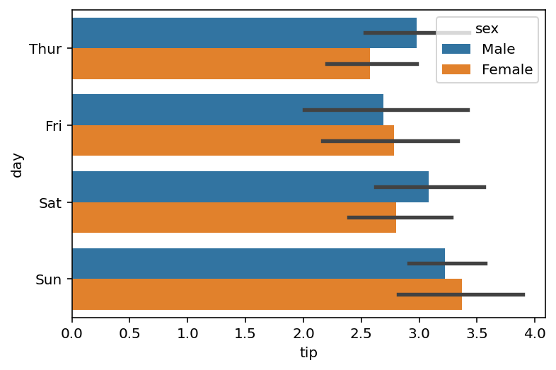
Dealing with A number of Teams with hue

When coping with information containing a number of teams, the hue parameter in seaborn.barplot() permits for creating grouped horizontal bar charts:

# Pattern information with teams
information = 'Class': ['A', 'B', 'C', 'A', 'B', 'C'],
        'Worth': [10, 25, 15, 12, 28, 18],
        'Group': ['X', 'X', 'X', 'Y', 'Y', 'Y']
df = pd.DataFrame(information)

sns.barplot(x="Worth", y="Class", hue="Group", information=df, palette="Set2")
plt.present()

This code introduces a brand new column "Group" to the DataFrame. The hue="Group" argument instructs Seaborn to create separate bars for every group inside every class, enhancing the comparability throughout completely different teams.

Working with Bigger Datasets and Information Aggregation

For bigger datasets, instantly plotting all information factors may result in cluttered charts. In such circumstances, information aggregation is critical. Pandas offers highly effective instruments for this:

# Pattern giant dataset (change with your individual)
# ... (Assume a big DataFrame 'df_large' with columns 'Class' and 'Worth') ...

# Mixture information utilizing groupby and imply
aggregated_data = df_large.groupby('Class')['Value'].imply().reset_index()

sns.barplot(x="Worth", y="Class", information=aggregated_data)
plt.present()

This instance demonstrates utilizing groupby() and imply() to mixture the info earlier than plotting, making certain a transparent and concise visualization even with numerous information factors. Different aggregation features like sum(), median(), or customized aggregation features can be utilized relying on the evaluation objective.

Including Annotations and Labels

Additional enhancing readability includes including annotations on to the bars, displaying the precise values:

ax = sns.barplot(x="Worth", y="Class", information=df)
for p in ax.patches:
    ax.annotate(f'p.get_width():.1f', (p.get_width(), p.get_y() + p.get_height() / 2.),
                ha='left', va='heart', xytext=(5, 0), textcoords='offset factors')
plt.present()

This code iterates by every bar (ax.patches) and provides an annotation displaying the bar’s worth utilizing ax.annotate(). The xytext parameter adjusts the annotation’s place relative to the bar.

Superior Strategies and Customization

Past the fundamental functionalities, Seaborn gives additional customization potentialities:

• Logarithmic Scale: For information spanning a number of orders of magnitude, utilizing a logarithmic scale on the x-axis can enhance readability. That is achieved utilizing plt.xscale('log').
• Customizing Tick Labels: Exact management over tick labels could be achieved utilizing plt.xticks() and plt.yticks().
• Including Legends: For charts with a number of teams (hue), a legend is mechanically generated. Its place and look could be personalized utilizing Matplotlib’s legend features.
• Saving the Plot: As soon as the chart is finalized, it may be saved to a file utilizing plt.savefig("filename.png").

Conclusion

Seaborn’s barplot() perform offers a versatile and highly effective software for creating horizontal bar charts, enabling efficient visualization of categorical information. By mastering the varied customization choices and understanding the underlying statistical rules, customers can generate insightful and aesthetically pleasing visualizations to speak information successfully. This complete information has explored the basic points of making and customizing these charts, from fundamental implementation to superior strategies, empowering customers to leverage the total potential of Seaborn for information visualization. Keep in mind to at all times contemplate your viewers and the precise message you wish to convey when selecting the suitable customizations in your horizontal bar chart. By combining the statistical energy of Seaborn with the visible customization choices of Matplotlib, you may create compelling visualizations that successfully talk your information insights.

Closure

Thus, we hope this text has offered helpful insights into Mastering Seaborn’s Horizontal Bar Chart: A Complete Information. We thanks for taking the time to learn this text. See you in our subsequent article!