Stacked Space Charts In R: A Complete Information

Stacked Space Charts in R: A Complete Information

Associated Articles: Stacked Space Charts in R: A Complete Information

Introduction

With enthusiasm, let’s navigate by the intriguing matter associated to Stacked Space Charts in R: A Complete Information. Let’s weave fascinating info and provide contemporary views to the readers.

Stacked Space Charts in R: A Complete Information

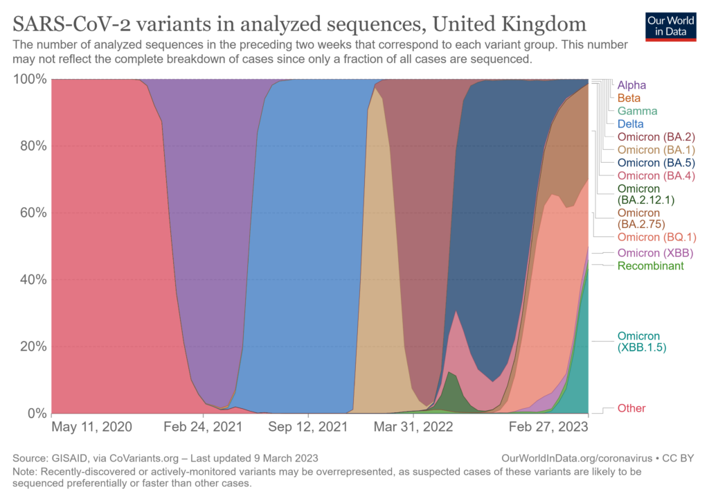
Stacked space charts are a robust visualization instrument used to show the composition of a complete over time or throughout classes. They excel at displaying the relative contribution of particular person elements to a complete, making them splendid for showcasing tendencies and proportions inside complicated datasets. This complete information will delve into the creation and customization of stacked space charts utilizing R, protecting varied packages, methods, and finest practices.

Understanding Stacked Space Charts

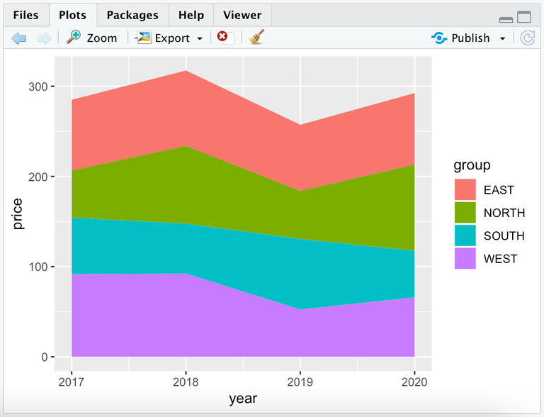
A stacked space chart represents knowledge as a collection of stacked areas, the place every space corresponds to a distinct class or element. The vertical axis represents the magnitude of the worth, whereas the horizontal axis represents time or one other categorical variable. The full peak of the stacked areas at any level alongside the horizontal axis represents the sum of all elements at that time. This permits for simple comparability of particular person elements’ contributions to the general whole and the identification of tendencies over time.

R Packages for Creating Stacked Space Charts

R affords a number of packages able to producing stacked space charts. Among the many hottest are:

• ggplot2: A part of the tidyverse, ggplot2 offers a grammar of graphics, providing a versatile and stylish strategy to knowledge visualization. It is extensively thought of the gold commonplace for creating high-quality and customizable plots in R.

• plotly: This package deal extends ggplot2‘s capabilities by creating interactive charts. Interactive stacked space charts created with plotly permit customers to hover over particular areas to see detailed info, zoom in on particular time intervals, and discover the info dynamically.

• lattice: lattice offers a robust different to ggplot2, providing a distinct strategy to graphics development. Whereas much less intuitive for freshmen, it offers appreciable flexibility and management over plot aesthetics.

• base R: Whereas much less visually interesting and versatile than devoted plotting packages, base R affords fundamental performance for creating stacked space charts utilizing capabilities like matplot. This may be helpful for fast visualizations or when working with quite simple datasets.

Creating Stacked Space Charts with ggplot2

ggplot2 is the popular alternative for a lot of R customers attributable to its versatility and intuitive syntax. The core perform is geom_area(), which is used to create space plots. The fill aesthetic is essential for assigning completely different colours to completely different classes, creating the stacked impact.

Let’s contemplate a pattern dataset representing gross sales of various product classes over a number of months:

library(ggplot2)
library(tidyr)

knowledge <- knowledge.body(
  Month = rep(month.abb[1:6], 3),
  Class = issue(rep(c("A", "B", "C"), every = 6)),
  Gross sales = c(10, 15, 20, 25, 30, 35, 12, 18, 24, 30, 36, 42, 8, 12, 16, 20, 24, 28)
)

# Reshape knowledge for ggplot2
data_long <- knowledge %>% pivot_wider(names_from = Class, values_from = Gross sales)

# Create the stacked space chart
ggplot(knowledge, aes(x = Month, y = Gross sales, fill = Class)) +
  geom_area() +
  labs(title = "Gross sales by Class Over Time", x = "Month", y = "Gross sales", fill = "Class") +
  theme_bw()

This code first masses the required libraries (ggplot2 and tidyr for knowledge manipulation). Then, it creates a pattern dataset. pivot_wider transforms the info right into a format appropriate for ggplot2. Lastly, it makes use of ggplot2 to create the chart, specifying the aesthetics (x, y, fill), including a title and labels, and making use of a black and white theme (theme_bw()).

Customizing ggplot2 Stacked Space Charts

ggplot2 affords intensive customization choices. We will modify:

• Colours: Use scale_fill_manual() to specify customized colours for every class.
• Labels: Modify axis labels and the title utilizing labs().
• Theme: Apply completely different themes utilizing capabilities like theme_classic(), theme_minimal(), or theme_bw().
• Legends: Customise the legend’s place and look utilizing theme() and legend.place.
• Aspects: Create a number of stacked space charts based mostly on one other variable utilizing facet_wrap() or facet_grid().
• Strains: Add traces to focus on the full or particular person element tendencies utilizing geom_line().

Instance with customization:

ggplot(knowledge, aes(x = Month, y = Gross sales, fill = Class)) +
  geom_area() +
  scale_fill_manual(values = c("A" = "blue", "B" = "inexperienced", "C" = "purple")) +
  labs(title = "Gross sales by Class Over Time", x = "Month", y = "Gross sales", fill = "Product Class") +
  theme_classic() +
  theme(legend.place = "backside")

This instance makes use of scale_fill_manual() to assign particular colours, adjustments the legend title, applies a basic theme, and strikes the legend to the underside.

Creating Stacked Space Charts with plotly

plotly builds upon ggplot2 to create interactive charts. The method could be very related, however we use ggplotly() to transform the ggplot2 object into an interactive plot.

library(plotly)

p <- ggplot(knowledge, aes(x = Month, y = Gross sales, fill = Class)) +
  geom_area() +
  labs(title = "Interactive Gross sales by Class", x = "Month", y = "Gross sales", fill = "Class")

ggplotly(p)

This code creates the identical chart as earlier than however converts it to an interactive plot utilizing ggplotly(). The ensuing chart will permit customers to hover over areas for detailed info and zoom and pan.

Dealing with Lacking Information

Lacking knowledge could cause points in stacked space charts. ggplot2 handles lacking knowledge by default, however it’s essential to know the way it’s dealt with. Lacking values will create gaps within the chart. Take into account imputation methods (e.g., utilizing the mice package deal) if lacking knowledge is substantial and impacts the interpretation.

Decoding Stacked Space Charts

When deciphering stacked space charts, give attention to:

• Relative Contributions: Observe the relative sizes of the areas to know the contribution of every class to the full.
• Developments Over Time: Establish tendencies in particular person classes and the general whole.
• Modifications in Composition: Search for shifts within the relative contributions of classes over time.
• Potential Outliers: Examine uncommon spikes or dips in particular person classes.

Conclusion

Stacked space charts are a helpful instrument for visualizing the composition of knowledge over time or throughout classes. R, notably with ggplot2 and plotly, offers highly effective and versatile instruments for creating and customizing these charts. By understanding the underlying rules and using the customization choices, customers can create informative and visually interesting visualizations that successfully talk complicated knowledge relationships. Keep in mind to all the time contemplate the context of the info and select the suitable chart kind and customization choices to finest characterize the knowledge and facilitate clear interpretation.

Closure

Thus, we hope this text has supplied helpful insights into Stacked Space Charts in R: A Complete Information. We thanks for taking the time to learn this text. See you in our subsequent article!